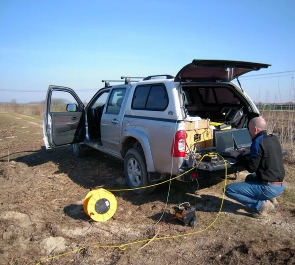
Brampton’s subsurface often hides surprises—buried channels, uneven shale bedrock, and pockets of saturated till that can skew a standard geotechnical investigation. Seismic tomography cuts through the guesswork: we use both refraction and reflection wave paths to build a continuous velocity profile of the ground, not just a single-location log. In the Chingacousy Creek corridor, for instance, we’ve mapped buried valleys that site drillers completely missed on the first pass. The technique works by generating a controlled seismic pulse—typically a sledgehammer or weight drop—and recording arrival times along a geophone spread. Refraction picks the critical refracted wave travelling along the top of competent bedrock; reflection captures deeper impedance contrasts, useful in Brampton’s glacial stratigraphy where till overlies shale at 15 to 40 metres depth. When the data is processed with tomographic inversion, the result is a 2D cross-section that shows lateral changes, fracture zones, and the true bedrock surface without interpolation. For projects near the Brampton Fair Grounds or along Steeles Avenue where fill thickness can jump 4 metres in under 20 metres of lateral distance, that continuous image is the difference between a confident design and an expensive revision order.
In Brampton’s glacial terrain, a tomographic velocity cross-section reveals the true bedrock surface—not an interpolated guess—and exposes buried channels that point data alone will miss.
How we work
The Halton Till that blankets most of Brampton is an overconsolidated silty clay with abundant clasts—great for bearing capacity but notoriously difficult for seismic ray penetration when dry and fractured. Summer surveys in July and August, when the upper 1.5 metres desiccates, often require a heavier energy source and tighter geophone spacing to maintain signal quality. We run 24- or 48-channel spreads with 2–5 metre receiver intervals depending on target depth; for a typical 30-metre bedrock investigation, a 115-metre spread with a midpoint shot and two off-end shots gives clean first breaks down to the shale interface. Tomographic processing uses curved-ray tracing rather than layered assumptions—critical in Brampton where the till-bedrock boundary is rarely planar. Where the overburden is saturated, we complement the P-wave dataset with a
MASW survey on the same spread to extract shear-wave velocities for seismic site class determination per NBCC 2020. On large linear corridors, such as the proposed transit extensions, combining seismic refraction with
resistivity profiling helps distinguish clay-rich till from sand lenses that could act as preferential drainage paths. Every line is processed to ASTM D5777-18 standards, with first-break picks verified independently by two analysts before inversion.
Local considerations
Brampton sits on the edge of two geological provinces: the thick Halton Till plain to the north and the glaciolacustrine silts closer to the Lake Ontario basin. That transition creates abrupt lateral changes in seismic velocity—a spread half on dense till and half on softer silt yields a velocity model that’s easy to misinterpret if processed with a 1D layered assumption. Spring thaw is another hazard. Late March and early April see the upper till fully saturated; the water table can rise to within 0.5 metres of the surface in low-lying areas near the Etobicoke Creek floodplain. In those conditions, the P-wave velocity of the near-surface jumps above 1,500 m/s, masking the true water table and hiding a thin, low-velocity layer that only a shear-wave survey or a carefully placed shot below the saturated zone would catch. Construction dewatering near deep excavations can also shift the velocity field mid-project—repeat lines before and after pumping are sometimes the only way to verify that the ground hasn’t changed. Overlooking these seasonal and anthropogenic effects leads to bedrock contours that are off by 2–3 metres, enough to change a footing design or a trenchless crossing profile.
Common questions
How deep can seismic refraction see in Brampton’s glacial soils?
With a 115-metre spread and a sledgehammer source, we typically image to 25–30 metres in dry summer conditions and 20–25 metres when the near-surface till is saturated. For deeper targets—such as shale bedrock below 35 metres—we switch to a weight-drop source and extend the spread to 230 metres or add a reflection component, which can reach 60+ metres with good resolution.
What does a seismic tomography survey cost for a typical Brampton site?
Can you run seismic lines on paved surfaces like parking lots or roads?
Yes. Geophones can be mounted on pavement using base plates and petroleum-jelly couplant; shot points on asphalt use a striker plate. The data quality on compacted pavement is often excellent because the plate-to-ground contact is repeatable. We do need to avoid buried utilities under the shot point, so a pre-survey locate is mandatory.
What’s the difference between refraction tomography and a standard refraction survey?
Standard refraction assumes the subsurface is a stack of flat, constant-velocity layers and computes a single velocity per layer. Tomographic inversion divides the ground into a grid of small cells and solves for the velocity in each cell using curved ray paths. In Brampton’s irregular till-bedrock interface, tomography recovers the true bedrock shape—especially important where the surface dips, pinches out, or contains buried valleys—while layered refraction often smooths or misplaces those features.